A Ceiling That Moved: skeg 0.6.0

A vector database has to keep a query cheap and its answer good as the corpus grows, and the corpus is exactly what makes both harder. This is a record of where skeg’s 0.6.0 line holds that, where it did not, and where a later change reversed a conclusion I had written down as final.

There are three parts. The first is a filtered query’s cost, which now follows the query’s neighbourhood instead of the size of the match set. The second is the recall of the 1-bit quantization tier, which I first measured as a ceiling: tq1 holds the top ten but slides on the top hundred as the corpus grows, and then, after changing how the graph is walked rather than how the vector is stored, measured again as flat to a million vectors. The third is what happens when many tenants share a box, where the cheapest architecture turned out to be the one that keeps them apart.

As in the earlier posts in this series, the intent is to report what was measured under the conditions the system was built for, and to name what was not. More of this post than I would like is a correction of numbers I had reported wrong or claimed too confidently, which is the other reason to write them down.

Part one: a filter’s cost ¶

A vector search with a filter answers two questions at once, which vectors are near the query and which satisfy a predicate on their metadata. The easy version, a predicate that matches almost everything, does not decide an architecture. The hard version is a filter that selects a large but proper subset of the corpus, scattered through the embedding space, at a size where touching every match is no longer free.

The exact way to serve it is to score every matching vector against the query and keep the top $k$. skeg has a cheap version of that: score each match with the in-RAM quantized proxy (a NEON-fast pass over 1-to-4-bit codes), then re-rank a small number of the best from the full-precision vectors on disk. The disk reads are bounded, so for a selective filter, a few thousand matches, it is fast and its result is exact.

The problem is the word every. The proxy scan is $O(|S|)$ in the size of the matching set $S$. On mxbai 1024-dim embeddings a 10% filter costs about 1.6 ms at 100k vectors, about 15 ms at 500k, and the line keeps climbing. A cost that grows with the data is the one you cannot ship, because the data is the thing that grows. The exactness is real; the scaling is the enemy.

Two things that did not survive ¶

The first instinct was to make the graph itself filter-aware. A label-aware Vamana build [1], the Filtered-DiskANN line [2], attaches the payload labels to the graph edges so the walk prefers paths through matching vectors. In an in-memory, exact-distance prototype it reached recall@10 of 0.99 at a narrow beam. It did not survive contact with skeg’s serving path. skeg walks the graph on the quantized proxy, not full precision, and on that proxy the label-aware graph plateaued below the plain scan it was meant to beat: about 0.985 at a 10% filter, 0.75 at 1%. It was cut. The lesson was specific and I paid for it more than once this cycle: a candidate mechanism has to be validated on the proxy path, because the proxy is what actually runs, not on the exact distances that make a prototype look good.

The second, a filtered graph walk with two complementary passes (one through the matching subgraph, one over the whole graph filtered at re-rank), holds recall when the matching vectors cluster together, the common case. It weakens when the matches are sparse and scattered, and it does not change the shape of the cost at low selectivity.

The route ¶

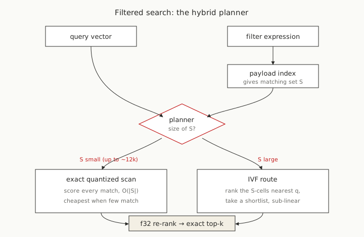
What shipped is a coarse index over the corpus, an IVF partition [3]: a few thousand k-means cells, no per-vector graph, roughly $\sqrt{N}$ cells. Each vector knows its cell; the whole structure is one centroid table plus one u32 per vector. A filter’s matching set S is not one cell but a scatter across many of them.

To serve a broad filter, the matching set is bucketed into its cells with a cheap $O(|S|)$ pass, those cells are ranked by their distance to the query, and the query-nearest cells that hold matches are gathered into a short list, which is then proxy-scored and f32 re-ranked.

The step that carries the design is the ranking: it ranks only the cells that actually contain a match, not the cells globally nearest the query. A naive IVF search ranks the query-nearest cells and probes those. That fails a filter whose matches cluster away from the query, because the nearest cells hold no matches and the probe returns nothing useful. Ranking the cells by their own membership in the match set fixes it. This is the whole of the probe, from the shipped code:

pub fn probe(&self, query: &[f32], s: &[u64], budget: usize) -> Vec<u64> {
    if s.len() <= budget {
        return s.to_vec();
    }
    // Bucket s into the cells that hold it (O(|s|) cheap lookups).
    let mut by_cell: AHashMap<u32, Vec<u64>> = AHashMap::new();
    for &id in s {
        let c = self.cell_of[id as usize];
        by_cell.entry(c).or_default().push(id);
    }
    // Rank the S-cells by query-centroid cosine (highest = nearest).
    let mut cells: Vec<(f32, u32)> = by_cell
        .keys()
        .map(|&c| {
            let ce = &self.centroids[c as usize * self.dim..c as usize * self.dim + self.dim];
            (cosine_f32(query, ce), c)
        })
        .collect();
    cells.sort_unstable_by(|a, b| b.0.total_cmp(&a.0));
    // Gather members from nearest S-cells until the budget is met.
    let mut out: Vec<u64> = Vec::with_capacity(budget + s.len() / self.n_cells.max(1));
    for (_, c) in cells {
        out.extend_from_slice(&by_cell[&c]);
        if out.len() >= budget {
            break;
        }
    }
    out
}

The pass over by_cell.keys(), not the full centroid table, is the design: only the cells that hold a match are ever scored against the query. That one choice is the difference between a route that finds an away-clustered filter and one that misses it.

This is not a small correction. In an isolated test on a correlated filter, one whose matching vectors sit in a region away from the query, query-centric probing recovered recall 0.69 while predicate-aware probing recovered about 1.00, at the same probe budget. The routing costs a bucket-and-rank over $S$, work the planner already has to do, not a second search.

Why it stays flat ¶

Take the numbers concretely. At 500k vectors the partition has about $\sqrt{500{,}000} \approx 707$ cells, roughly 700 vectors each. A 10% filter is 50,000 matches, scattered across most of those cells. The scan touches all 50,000. The route, with a shortlist budget of 4,096, gathers from the six or so query-nearest cells that hold matches and stops. The cost is proportional to the shortlist, a fixed budget, not to the 50,000 matches. That is the whole trick: the work follows the query’s neighbourhood, not the size of the filter.

The planner picks between the two by the absolute size of the match set, not a fraction of the corpus. Below about 12,000 matches the exact scan is cheaper than the route’s fixed overhead, so the planner scans; above it, the route wins. Because the crossover is in absolute matches, it holds at any corpus size: a small filter is small whether the corpus is 100k or 10M.

The routing index is built off the request path, during the background idle consolidate, and persisted in a sidecar next to the graph, so it survives a restart and adds nothing to query latency. Measured on mxbai 500k over the disk-and-proxy path the engine actually runs:

selectivity	matches	IVF route (recall@10 / ms)	scan every match
1%	5k	1.00 / 1.1 ms	1.00 / ~1 ms
10%	50k	0.99 / 2.6 ms	1.00 / 15 ms
50%	250k	0.96 / 5.5 ms	1.00 / 53 ms

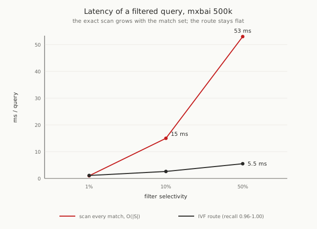
The scan stays exact and climbs to 53 ms at 50%. The route stays at a few milliseconds and trades a small recall margin, tunable through the shortlist budget, for a cost that does not grow. At 1% both paths are cheap and the planner picks the scan, which is exact. The gain is entirely in the regime where the old answer was getting expensive. The shortlist budget is the one knob here, and it returns in part three with a bill attached: the same route that keeps a filter’s cost flat is what caps a filtered tenant’s recall when the match set gets large.

The cost of building it ¶

The router is built during the background consolidate, the same pass that folds buffered writes into the on-disk graph. That pass is dominated, about 90% of it measured, by the graph build itself, and the graph build’s cost scales with its search width l_build. The in-RAM index builds at width 64. The disk path in 0.6.0 drops the default to 48. A sweep on mxbai 100k picked the number: 48 holds recall@10 (0.994 against 0.9955 at 64) while cutting the graph build by about 24%. Because the build dominates consolidate, and consolidate dominates a bulk ingest, that 24% shows up directly as faster ingest, for a fifth of a percent of recall the re-rank largely gives back anyway. This is the same lesson as the route, from the other direction: the cheap win is picking the width that the data says is enough, not the width that looks safe.

Part two: what the answer costs, and a ceiling that moved ¶

The other thing that is supposed to hold is recall. skeg keeps the full vectors on SSD and walks the graph on a quantized proxy, then re-ranks the survivors against the full precision. The tier is the proxy: TurboQuant [4] at 1, 2, or 4 bits per coordinate. TurboQuant is a data-oblivious quantizer: it compresses each vector to a handful of bits per dimension with a fixed random rotation and no trained codebook, so unlike a learned method (OPQ, PQ [3]) it never goes stale under live writes: there is nothing to retrain when the data shifts. That property is the reason it is the tier at all.

tq1 (1 bit) is the cheapest: it stores one sign bit per rotated coordinate, half the RAM of tq2 again. The question this cycle was whether tq1 is good enough to be the quiet default for everyone. I answered it wrong twice (once with a flattering metric, then once with the right metric but the wrong navigation), and the second mistake is the interesting one.

A number I was reporting wrong ¶

Before anything, the metric. For most of this cycle I reported tq1 at “recall@100 around 0.996” and felt fine about it. The number was measured by a harness that searched for the top 10, then checked how many of those 10 fell inside the true top 100. That is not recall@100. It is “how many of my top 10 are broadly relevant,” and it reads near 1.0 for almost any half-working index. It hid the thing it was named after.

Recall@100 is a top-100 search compared against the true top 100. When I finally measured that, on real $k=100$ searches against a brute-force ground truth, the picture changed. The metric had been flattering, I trusted it across a lot of runs, and it took a pointed question to make me search for the top 100 instead of the top 10.

The ceiling I first measured ¶

Here is what the real metric showed at the default beam, with the proxy tq1 was then walking on: a symmetric Hamming popcount, query and vector both reduced to one bit:

corpus	tq1 @10	tq1 @100
20k	0.987	0.938
100k	0.993	0.893
500k	0.978	0.843

Read the second column. tq1 holds recall@10 well but its recall@100 slides from 0.94 to 0.84 as the corpus grows. The reading I wrote down, and shipped as the positioning for 0.6.0, was that this is intrinsic: a 1-bit code has coarse discrimination, so as the corpus grows more vectors sit within one bit’s worth of each other, the true top 100 no longer surface in a fixed-budget walk, and the honest move is to make tq1 the economy tier for small tenants and point broad retrieval at tq2. Widening the walk recovered the recall but cost the latency tq1 was supposed to save. That was the conclusion. It was wrong, and the reason it was wrong is that I had blamed the code for a limit that belonged to the proxy metric.

The distinction I had collapsed ¶

A 1-bit code and a 1-bit distance are not the same thing. The vector is stored as one sign bit per coordinate; that is fixed. But the query need not be. skeg had been walking on a symmetric popcount (query also reduced to sign bits, distance is the Hamming count of disagreements), which is fast (one XOR-and-popcount per candidate) but throws away everything about how far the query sits from the splitting plane on each axis. That is the coarseness. It is a property of the comparison, not of the stored bits.

Two facts, measured, pin this down. First: on glove (a low-dimensional set where 1-bit navigation struggles most), the same graph navigated on an int8 proxy reaches recall@100 of 0.945 at a narrow beam where the 1-bit popcount reaches 0.58. The true neighbours are reachable in the graph; the popcount metric just cannot steer to them. Second: giving the query full f32 precision against the same 1-bit stored code (an asymmetric distance, the RaBitQ [5] construction) lifts mxbai 100k recall@100 from 0.893 to 0.970 at the default beam, no change to storage. The stored bit was never the ceiling. The symmetric comparison was.

Bit-plane: an asymmetric distance that stays integer ¶

Full f32 on the query works but is slow: it puts a floating-point multiply-add on every candidate in the hot walk, and a measured 9× loss in throughput for a few points of recall is the wrong trade. What shipped instead keeps the query in integers. Quantize the rotated query to $B$ bits and transpose it into $B$ bit-planes; the inner product against a stored sign code is then $B+1$ integer popcounts, no floating point per candidate. This is the multi-bit-query trick from the TurboQuant notes [4]; the algebra is worth writing out because it is the whole mechanism.

The stored code is the sign pattern $s_i = \operatorname{sign}(Rx)_i \in \{-1,+1\}$ of the rotated unit vector, and its 1-bit reconstruction is $c\,s_i$ with $c = \sqrt{2/\pi}\,/\sqrt{d}$, the Lloyd-Max level for a unit-variance Gaussian coordinate. Scalar-quantize the rotated query to $B$ bits, $q_i \approx m + \Delta\,Q_i$ with $Q_i \in [0, 2^B-1]$, minimum $m$ and step $\Delta$. Then the estimator splits into two integer sums:

$$\langle q, s\rangle \;=\; \sum_i q_i s_i \;=\; m\sum_i s_i \;+\; \Delta\sum_i Q_i s_i .$$

Both sums are popcounts. Writing $\text{pc}(\cdot)$ for population count and $\text{plane}_b$ for the bit-mask of query coordinates whose $b$-th bit is set,

$$\sum_i s_i = 2\,\text{pc}(\text{code}) - d, \qquad \sum_i Q_i s_i = 2\sum_{b=0}^{B-1} 2^{b}\,\text{pc}(\text{plane}_b \wedge \text{code}) \;-\; \textstyle\sum_i Q_i ,$$

because $s_i = 2\,[\text{code}_i{=}1] - 1$ and $Q_i = \sum_b 2^b\,\text{bit}_b(Q_i)$. The per-candidate cost is one popcount for $\text{pc}(\text{code})$ plus one per plane ($B+1$ in total) with the query scalars $m$, $\Delta$, $\sum Q_i$ computed once. As $B \to \infty$ this converges exactly to the f32 asymmetric estimator; at finite $B$ it is a strictly integer approximation of it. The scoring is done in a fixed-point contract, c times the reconstruction times the per-vector norm correction skeg already stores, so it slots into the existing proxy without a new code path.

$B$ is the one dial. On mxbai 100k, recall@100 goes 0.911 at $B{=}2$, 0.960 at $B{=}3$, 0.967 at $B{=}4$, against the f32-asymmetric ceiling of 0.970. $B{=}4$ is the knee (within a fifth of a percent of full precision, four popcounts a candidate), and it is the default. It replaces both the pure popcount and a dimension-keyed switch that used to pick asymmetric only above 512 dimensions: one navigation mode, no dimensional special-casing.

The curve that moved ¶

With the bit-plane walk and a beam tuned to what the metric needs (search width 1000, re-rank budget 3200), the ceiling I had written down as intrinsic is gone. Every number below is a clean single-tenant run, one process at a time, no contention:

embedding	dim	N	recall@10	recall@100	p50	p99	RAM idle	QPS
minilm	384	100k	0.9955	0.9939	2.7 ms	3.6 ms	32 MB	941
mnist	784	60k	0.9990	0.9956	2.0 ms	2.5 ms	22 MB	870
qwen3	2560	20k	1.0000	0.9996	3.6 ms	4.2 ms	12 MB	856
mxbai	1024	100k	1.0000	0.9990	3.0 ms	3.8 ms	40 MB	860
mxbai	1024	500k	1.0000	0.9979	2.8 ms	4.8 ms	198 MB	864
mxbai	1024	1M	0.9995	0.9969	7.6 ms	33 ms	397 MB	830

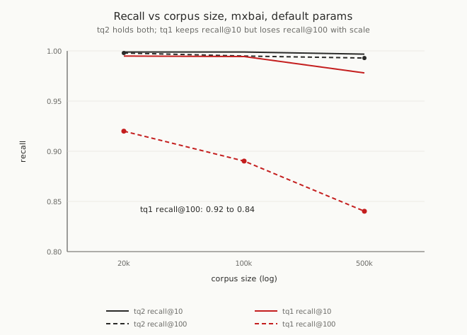
Recall@100 holds above 0.996 to a million vectors at 1-bit storage, on the tier that was the economy option. The RAM is the index resident set (graph plus 1-bit codes), and it is what the tier was for: roughly 400 bytes a vector, the f32 copies stay on SSD. The one number to read honestly is the 1M p99, 33 ms against a p50 of 7.6: that tail is the re-rank reading cold pages of the 4 GB vectors.bin that do not all fit in page cache, disk I/O, not the walk; it falls back toward the p50 when the file is warm, which is the RAM/latency trade the next part is about.

Two dials, two bottlenecks ¶

The tuning is not one knob. Recall@100 is walk-limited: it moves with the search width and is flat against the re-rank budget: widen the walk to reach the true neighbours. Recall@10 is re-rank-limited at a deep walk: the top ten are already in the beam, and the budget decides how many get the exact f32 comparison that orders them. So the width buys the hundred and the budget buys the ten, and they are tuned against different curves. The defaults (1000 / 3200) sit where the worst dataset in the set clears 0.99 on both.

The one place the code still wins over the walk ¶

Not everything is navigation. glove is 100-dimensional; padded and stored at one bit, a vector is 104 bits, and no walk recovers what those bits never captured. At the common config it reads recall@100 of 0.79; only a very wide walk, at ~11 ms, reaches 0.95. That is a genuine storage limit at low dimension (the regime where 1-bit quantization has too little to work with), and the honest handling is a wider beam for that one case, paid in latency, not memory. It does not move the result for the embeddings the tier is actually for, dimension 384 and up, where the table above is the whole story.

Two things I tried that did nothing, recorded because they looked promising ¶

Twice I chased a lever that the data refused. Neither shipped; both are here because “I tried the obvious thing and measured it flat” is the point of these posts.

The first was a quantizer-aware graph build, the QuIVer construction [6]: run the Vamana pruning on the 1-bit popcount metric instead of f32, so the graph’s edges are the ones the popcount walk can actually follow. On paper it is exactly the fix for a topology mismatched to its proxy. Measured on mxbai it moved recall@100 by 0.002, inside the noise, because skeg’s f32-built graph is already navigable by the proxy; the bottleneck was the metric mis-ranking within the beam, which the bit-plane fixes and a rebuilt graph does not.

The second was anisotropy compensation, a per-coordinate shift and scale learned from the rotated distribution, the trick TurboQuant’s notes credit with several points at 1 bit, related to the score-aware objective in ScaNN [7]. Folded onto the asymmetric query it should have lifted the anisotropic sets. Full shift-plus-scale collapsed recall (a mean-heavy coordinate drove the per-vector norm correction toward zero); scale-only was stable and flat. The reason it does nothing here is specific and worth keeping: skeg’s asymmetric path already carries an f32 query and an $\lVert v\rVert/\langle\cdot\rangle$ renormalization, so the headroom the compensation is supposed to fill is already filled. A trick that pays on an 8-bit quantized query has nothing left to recover on a full-precision one.

Part three: many tenants on one box ¶

A multi-tenant deployment is where the memory story and the filter story collide. The obvious design is one shared index with a tenant= field on every vector and a filtered query per tenant; it reuses the filter route from part one, and it looks like the frugal choice. Measured, it is the wrong one, and for a reason that is the exact bill of that route.

The filtered path narrows through the IVF shortlist, budget 4,096. With five tenants of 20k that is fine, but a tenant’s match set grows with the tenant, and at 100k matches the shortlist of 4,096 is a small fraction of the candidates: the true neighbours are dropped before the re-rank ever sees them. Recall@100 falls off as the tenants grow:

model	tenants	N total	recall@10	recall@100	p50	QPS
shared + filter	5 × 20k	100k	0.992	0.973	3.4 ms	293
shared + filter	5 × 100k	500k	0.970	0.933	5.3 ms	292
shared + filter	5 × 200k	1M	0.961	0.922	8.0 ms	285
one index / tenant	5 × 20k	100k	1.0000	0.9997	1.7 ms	922
one index / tenant	5 × 100k	500k	1.0000	0.9990	2.0 ms	926
one index / tenant	5 × 200k	1M	1.0000	0.9988	2.2 ms	895

An index per tenant wins on every axis, and it wins for structural reasons, not tuning. Each tenant is served by the graph walk from part two, not the filter route, so its recall is the single-tenant recall, flat to 1M. Its graph holds only that tenant’s vectors, so the walk is shorter than the shared graph’s, and the p50 drops with it. The RAM total is identical: the same vectors and the same 1-bit codes, partitioned into separate graphs rather than one, with negligible per-index overhead. And isolation comes free: no tenant’s query can leak another’s vector, and a noisy tenant’s load lands on its own index. The shared-and-filtered model earns its keep only where tenants are many and tiny, or where a query must cross tenants; for tenants with real corpora, keeping them apart is both the higher-recall and the cheaper answer.

A note on memory, measured three ways ¶

The tier’s whole claim is a small resident footprint, so it is worth being precise about which number that is. There are three, and they are not equal.

The index resident set (graph plus 1-bit codes, what skeg logically holds) is the small one: 40 MB at mxbai 100k, 400 MB at 1M, linear in the corpus, the f32 vectors on disk. The server RSS is larger: measured on the real server it runs ~100 MB over the index for small corpora and tapers as the index grows (120 MB at 100k, 240 MB at 500k, 427 MB at 1M), the gap being the runtime (allocator, thread pool, buffers), not the data. And the hot RSS under query load adds the pages of vectors.bin the re-rank touches, which on this platform live in the kernel’s page cache, outside the process’s own resident set, which is why the server RSS reads about the same warm as cold.

0.6.0 also lets the quantized codes be memory-mapped from a file instead of held in owned RAM, and I owe a correction here too. The intuition was that this lowers the serving footprint. In a hot query loop it does not; the walk touches most of the codes, they page in, and the resident set matches owned RAM. What mmap actually buys is reclaimability: the codes are file-backed, so the OS can drop a cold or contended index’s pages and read them back on demand without swap. On the multi-tenant box of part three this is the lever the linear-RAM table hides: the resident tables report every tenant fully held, but with mmap the idle tenants’ pages fall out of RSS and the warm ones stay, so the memory a packed box insists on keeping tracks the working set, not the sum. It lowers the memory an idle index insists on, not the memory a hot one uses. It is not a way to get tq2’s discrimination at tq1’s footprint, which is the thing I briefly, wrongly, implied it was: that turned out to be a job for the walk, not the storage.

What this record supports ¶

Three findings, each narrow.

A filtered query’s cost can be made to follow the query’s neighbourhood rather than the size of the match set. The route that does it is exact where the scan is cheap and a bounded approximation where it is not.

The 1-bit tier’s recall@100 ceiling was never the stored code. It was the distance I compared against it. An integer bit-plane estimator, the query in $B$ bits against the vector’s one, holds recall@100 above 0.996 to a million vectors at 1-bit storage. That is the number I had written off as needing tq2.

And for many tenants on one box, an index each beats one index filtered, on recall and latency and cost together, with isolation falling out for free instead of being a thing to build.

The evidence is thinner than the conclusions, and I would rather be exact about how than round it up. The numbers are from one machine, one embedding family for the scale runs, and fixed query sets, reproducible only to within the hardware’s run-to-run noise. This cycle taught me what that noise can cost a reported figure: several latencies in my first pass, printed from a serialized re-run under contention, were three to twenty times too high before I caught and corrected them. This is not a third-party benchmark, and more of it than I would like is a record of being wrong first: a flattering metric, a ceiling that belonged to the walk and not the bit, an mmap win aimed at a problem it did not solve.

That last part is why the record is worth keeping. A number reported once and never checked again is indistinguishable from one that merely happened to be right; the correction is what tells them apart. So the value here is not the headline figures but that the retractions sit beside them. The route is shipped, the walk is changed, the tiers are placed, and the numbers left standing are the ones that survived being measured a second time.

---

References ¶

[1] Subramanya, Suhas Jayaram; Devvrit; Kadekodi, Rohan; Krishaswamy, Ravishankar; Simhadri, Harsha Vardhan. “DiskANN: Fast Accurate Billion-point Nearest Neighbor Search on a Single Node.” Advances in Neural Information Processing Systems 32 (NeurIPS 2019), 2019.

[2] Gollapudi, Siddharth; Karia, Neel; Sivashankar, Varun; Krishnaswamy, Ravishankar; Begwani, Nikit; Raz, Swapnil; Lin, Yiyong; Zhang, Yin; Mahapatro, Neelam; Srinivasan, Premkumar; Singh, Amit; Simhadri, Harsha Vardhan. “Filtered-DiskANN: Graph Algorithms for Approximate Nearest Neighbor Search with Filters.” Proceedings of the ACM Web Conference 2023 (WWW ‘23), 2023.

[3] Jégou, Hervé; Douze, Matthijs; Schmid, Cordelia. “Product Quantization for Nearest Neighbor Search.” IEEE Transactions on Pattern Analysis and Machine Intelligence, vol. 33, no. 1, 2011.

[4] Pleshkov, Ivan. “TurboQuant and RaBitQ: notes on a data-oblivious vector quantizer.” Engineering write-up, ivanpleshkov.dev/blog/turboquant. The tier is skeg’s own implementation of the TurboQuant family; this note is the closest public description of the tricks it builds on, including the multi-bit-query / bit-plane scoring used here.

[5] Gao, Jianyang; Long, Cheng. “RaBitQ: Quantizing High-Dimensional Vectors with a Theoretical Error Bound for Approximate Nearest Neighbor Search.” Proceedings of the ACM on Management of Data (SIGMOD), 2024. The asymmetric estimator (full-precision query against a 1-bit code) is the construction the bit-plane distance approximates in integers.

[6] “QuIVer: Rethinking ANN Graph Topology via Training-Free Binary Quantization.” Preprint, arXiv

.02171, 2026. Tested here (build the graph on the 1-bit metric) and measured flat on skeg’s already-navigable graph; recorded as a non-result.

[7] Guo, Ruiqi; Sun, Philip; Lindgren, Erik; Geng, Quan; Simcha, David; Chern, Felix; Kumar, Sanjiv. “Accelerating Large-Scale Inference with Anisotropic Vector Quantization.” Proceedings of the 37th International Conference on Machine Learning (ICML), 2020. The score-aware objective behind the anisotropy-compensation attempt that, on an already-asymmetric f32 query, had nothing to recover.