What Was Measured: The Numbers

The four posts before this one recorded the constraints, the falsifications, the substrate, and the surviving hypothesis. They argued for an architecture without measuring it against alternatives existing in the field. This record closes that gap. It reports the numbers from the benchmark suite run on the shipped configuration of the system, against five other engines for vector retrieval, on the same hardware, with the same ground truth, and under the same selection criterion.

The criterion is $\text{recall}@10$ against a brute-force ground truth, with a threshold of $0.95$. For each engine and at each configuration, the bench sweep selects the operating point achieving the highest throughput while clearing the recall threshold. Where no point clears it, the failure is recorded and the engine appears in the comparative tables with that note. The criterion is uniform across engines.

The numbers below are from a single bench run executed on 2026-05-22 against a development machine. They do not constitute a third-party benchmark. The run is reproducible to within the run-to-run noise of the hardware. The intent of this post is to record what was measured under the conditions the project was built for, specifying what was not measured and why.

---

Hardware and method ¶

The numbers in this record were collected on the development machine of the project: a MacBook Pro M1, 16 gigabytes of unified memory, macOS 26.2. The binary was compiled with -C target-cpu=apple-m1 -C target-feature=+neon,+dotprod using a nightly Rust toolchain.

The primary corpus is mxbai-wiki-chunked, a one-million-vector embedding of Wikipedia chunks produced with mxbai-embed-large-v1 at dimension 1024. A second corpus is used for the multi-distribution check: minilm-100k, 100,000 vectors of Wikipedia chunks at dimension 384 produced with all-MiniLM-L6-v2. The mxbai distribution is approximately isotropic on the unit sphere. The minilm distribution is lower-dimensional and exhibits a less uniform per-coordinate variance. Both represent the embedding geometries encountered in a personal AI deployment.

Seven engines were tested. Five are external: qdrant-hnsw, qdrant-sq, qdrant-pq, chroma-hnsw, and lancedb. Two are skeg in its shipping configurations as proxy tier defaults: skeg-int8 and skeg-pq128. The third skeg tier, TurboQuant, is omitted from the cross-engine comparison for reasons recorded in the caveats section. Each engine was tuned through its specific recall-latency knob: l_search for the Vamana family, ef for HNSW, and nprobes for IVF-PQ. The sweep was performed independently for each engine according to its official documentation.

The selection criterion across all comparisons is uniform: for each engine at each corpus scale, the sweep selects the point that achieves the highest throughput while meeting $\text{recall}@10 \ge 0.95$ against a brute-force ground truth. Where no sweep point meets the criterion, the point of highest recall is reported and flagged. The headline numbers below are reproducible to within the run-to-run noise of the machine recorded by the harness.

---

The headline: one million vectors at recall $\ge$ 0.95 ¶

The first measurement targets the configuration the project was built for: a single-node deployment of one million vectors of dimension 1024, served under single-stream load. The table below lists the sweep point meeting the recall criterion for each engine, ordered by resident memory.

engine	recall@10	p50 (ms)	p99 (ms)	qps	RSS (MiB)	disk (MiB)	build (s)
skeg-pq128	0.998	2.0	3.6	489	419	4162	918
skeg-int8	0.999	2.9	10.2	299	1252	4162	892
qdrant-sq	0.951	2.4	5.3	390	3023	532	3628
qdrant-hnsw	0.994	3.7	38.9	168	4162	4340	647
chroma-hnsw	0.983	4.8	9.7	196	4417	4215	2036

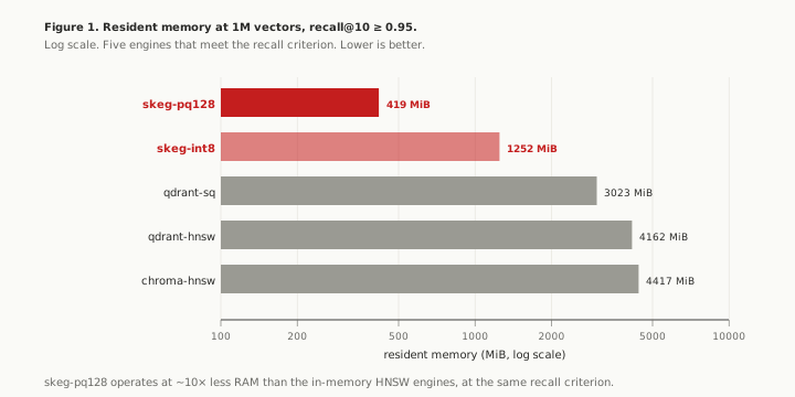
The resident memory of skeg-pq128 is 419 MiB. It operates the one-million-vector configuration in approximately one-tenth of the memory required by qdrant-hnsw (4162 MiB) or chroma-hnsw (4417 MiB). This meets the constraint envelope of the first post in this series: a personal AI deployment can hold a one-million-vector retrieval index resident alongside a five-gigabyte language model without exhausting system memory.

qdrant-hnsw returns the highest recall on the table ($0.994$) but its p99 is 38.9 milliseconds, against 3.6 milliseconds for skeg-pq128 and 9.7 milliseconds for chroma-hnsw. The HNSW path under single-stream load has a long tail at this scale, whereas the disk-resident Vamana path of skeg maintains a tight distribution.

skeg-pq128 reaches 489 queries per second at the same recall point. This falls below the throughput of an in-memory engine running with a hot cache and no memory pressure, which is outside the operating regime of a personal AI deployment, but it exceeds the throughput of the other engines on the table clearing the recall threshold.

Two engines warrant separate mention. qdrant-pq was included in the sweep but is absent from the table. At its tuned configuration it returned a $\text{recall}@10$ of $0.78$, falling below the $0.95$ criterion. The configuration of qdrant-pq was not optimized in this bench, and its omission reflects the criterion rather than a judgment on the engine. lancedb is also omitted due to the configuration anomalies detailed in the caveats section.

---

Scaling from 100K to one million ¶

The second measurement tracks engine scaling relative to corpus size. The same sweep criterion applies: for each engine at three scales (100K, 500K, 1M), the table reports the point achieving the highest throughput at $\text{recall}@10 \ge 0.95$.

engine	scale	recall@10	p99 (ms)	qps	RSS (MiB)
skeg-pq128	100K	1.000	2.4	587	63
skeg-pq128	500K	0.999	3.0	541	220
skeg-pq128	1M	0.998	3.6	489	419
skeg-int8	100K	1.000	2.3	603	131
skeg-int8	500K	0.999	2.9	608	635
skeg-int8	1M	0.999	10.2	299	1252
qdrant-hnsw	100K	0.995	3.3	374	878
qdrant-hnsw	500K	0.988	3.6	386	2337
qdrant-hnsw	1M	0.994	38.9	168	4162
qdrant-sq	100K	0.963	2.7	456	949
qdrant-sq	500K	0.954	3.2	442	2831
qdrant-sq	1M	0.951	5.3	390	3023
chroma-hnsw	100K	0.990	4.9	253	735
chroma-hnsw	500K	0.986	7.4	226	2419
chroma-hnsw	1M	0.983	9.7	196	4417

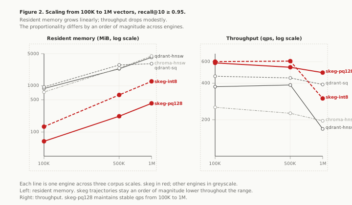
The resident memory of every engine scales linearly with corpus size, though the proportionality constants differ. At 1M, the two HNSW engines reach four gigabytes. The skeg engines require 419 megabytes and 1.25 gigabytes respectively. The disk footprint is uniform across engines and scales with the raw vector data rather than the index structure.

Recall behaviour remains stable across scales. Engines meeting the $0.95$ criterion at 100K continue to meet it at 1M, with absolute recall degradation staying below one percent.

Throughput trends split the engines into two groups. The skeg engines maintain stable throughput from 100K to 500K before separating at 1M. The HNSW engines drop more gradually but start from a lower baseline. The ratio between throughput at 100K and 1M is approximately $0.83$ for skeg-pq128, $0.50$ for skeg-int8, $0.45$ for qdrant-hnsw, $0.86$ for qdrant-sq, and $0.77$ for chroma-hnsw.

Tail latency differentiates the disk-resident Vamana path of skeg from the in-memory HNSW path of qdrant and chroma. At 1M, the p99 of qdrant-hnsw is 38.9 milliseconds, which is more than ten times its p50. The corresponding ratio for skeg-pq128 is $1.8$. The Vamana walk, combined with re-ranking against full-precision vectors on disk, yields a narrower latency distribution than HNSW under these operating conditions.

---

Recall versus latency at 500K ¶

The scaling section isolates one operating point per engine per scale. The recall-latency Pareto curve offers a broader view, mapping the trade-off between accuracy and tail latency across the complete sweep of each engine’s tuning knob. This is the baseline representation in approximate-nearest-neighbor literature, reported here at the intermediate 500K scale.

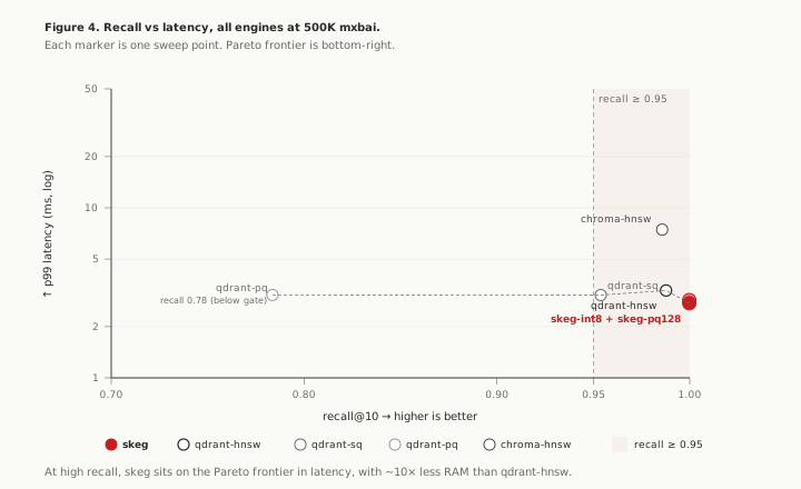
The Pareto frontier sits at the lower-right region of the plot, representing high recall and low latency. Two engines occupy this frontier at the recall-criterion line ($\text{recall} \ge 0.95$): skeg-int8 and skeg-pq128. Their operating points overlap, with p99 latencies within 5 percent of each other and recall values above $0.999$. To their left on the recall axis sit qdrant-hnsw ($\text{recall} = 0.99$) and qdrant-sq ($\text{recall} = 0.95$). In the upper section, chroma-hnsw reaches a recall of $0.99$ at a higher p99 latency. qdrant-pq falls outside the targeted recall band with a maximum tuned recall of $0.78$.

The position of skeg on the frontier matches the latency trends observed in the scaling section. At high recall points, the disk-resident Vamana path delivers tail latencies competitive with the in-memory HNSW path of qdrant. The memory metric separates them: skeg reaches the frontier at a fraction of the resident memory used by qdrant-hnsw. LanceDB is omitted from the plot for the reasons detailed below.

---

Concurrency ¶

The third measurement evaluates throughput under concurrent loads. At a fixed corpus scale of 100K vectors, the harness issues queries from a variable number of concurrent client threads: $1$, $4$, $16$, and $64$. For each engine and concurrency step, the point with the highest throughput meeting $\text{recall} \ge 0.95$ is selected.

The skeg engines scale throughput linearly from one to 16 concurrent clients, and show additional gains at 64. The two HNSW engines, qdrant-hnsw and chroma-hnsw, scale up to 16 threads and then plateau or regress. Their throughput at 64 matches or falls below their 16-thread baseline, while tail latencies expand. This indicates that the in-memory HNSW path encounters lock contention on graph nodes under high concurrency. The disk-resident Vamana path of skeg, utilizing per-shard worker pools and avoiding shared mutable state on the read path, avoids this contention surface. The explicit metrics and curves will reside in the repository notebook upon release.

---

Multi-distribution ¶

The prior tests used mxbai-wiki-chunked, an isotropic 1024-dimensional embedding. The fourth measurement verifies whether the relative performance ranking holds under a different embedding geometry. The corpus used is minilm-100k, a 384-dimensional embedding generated via all-MiniLM-L6-v2. This distribution features a lower intrinsic dimension and a less uniform per-coordinate variance.

The metrics at 100K, side-by-side:

engine	recall mxbai	recall minilm	qps mxbai	qps minilm	RSS mxbai (MiB)	RSS minilm (MiB)
skeg-int8	1.000	1.000	603	829	131	73
skeg-pq128	1.000	1.000	587	553	63	49
qdrant-hnsw	1.000	0.983	374	510	878	537
qdrant-sq	0.963	0.954	456	696	949	613
chroma-hnsw	0.990	0.982	253	363	735	499

The relative performance and resource rankings remain unchanged. Every engine registers higher throughput on minilm. A 384-dimensional dot product is roughly 2.7 times cheaper than a 1024-dimensional dot product, while the rest of the execution path remains uniform. The recall and memory hierarchies match the mxbai baseline.

The skeg engines show tighter resident memory footprints on minilm because the space savings from int8 and PQ scale directly with vector dimensionality. At 384 dimensions, the absolute memory allocation drops for all candidates, but skeg maintains its relative resource advantage.

---

Skeg internal: the five tiers ¶

The cross-engine data uses two shipping configurations of skeg: skeg-int8 and skeg-pq128. The runtime supports three additional tiers: TurboQuant at 1, 2, and 4 bits per coordinate. The internal trade-offs across these five tiers were recorded on a 100K mxbai corpus using a single tenant in default RAM mode.

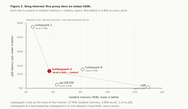
The Pareto-dominant configurations for resident memory and latency are turboquant-1, turboquant-2, and int8. On this dataset, pq:128:256 and turboquant-4 are dominated by turboquant-2, which provides equal or higher recall at lower or equivalent memory footprints along with competitive latencies.

The tier options, ordered by resident memory:

tier	RSS (MiB)	p50 (ms)	recall@10	notes
turboquant-1	45	2.9	0.996	smallest footprint, slowest
turboquant-2	57	1.3	0.999	default for multi-tenant
pq:128:256	63	0.8	0.996	default for single-tenant
turboquant-4	82	1.4	0.998	dominated by tq-2 here
int8	130	0.7	0.997	fastest, heaviest

turboquant-2 represents the knee of the trade-off curve for deployments where resident memory is the binding operational constraint and recall must remain near maximum. pq:128:256 retains a minor advantage in p50 latency at 100K and serves as the default configuration for single-tenant instances with wider RAM headroom. turboquant-4 is outmatched by turboquant-2 on this specific dataset. It remains available for embedding distributions with higher intrinsic dimensionality than mxbai, where the extra proxy bits affect accuracy. The design of TurboQuant and its promotion criteria were documented in the previous post.

---

Multi-tenant on disjoint corpora ¶

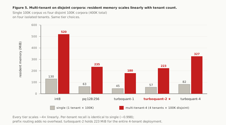
The fifth measurement focuses on the multi-tenant layout of the system. In slice M-F, the harness builds four disjoint 100K corpora from the same Wikipedia source (slices [0:100K], [100K:200K], etc.), computes an isolated ground truth for each, and runs four parallel tenants across four separated skeg instances. The combined corpus totals 400K vectors across the tenants. Each tenant runs a 1,000-query stream against its own index. Recall is evaluated per tenant and averaged.

Three operational properties were observed in this configuration.

First, per-tenant recall matches the single-tenant 100K baseline. Across all five tiers, multi-tenant $\text{recall}@10$ deviates from the single-tenant baseline by less than $0.001$, which is within the measurement noise of the harness. The prefix-routing isolation scheme does not lower retrieval quality.

Second, resident memory scales linearly with tenant count. At four tenants, total resident memory is roughly four times the single-tenant footprint: int8 moves from 130 MiB to 520 MiB, and turboquant-2 moves from 57 MiB to 223 MiB. The prefix-routing layer introduces no structural memory overhead beyond the data held by individual tenants.

Third, per-tenant latency at a concurrency of four is lower than single-tenant latency at a concurrency of one. The multi-tenant deployment executes four isolated server instances. Each operates at an effective concurrency of one, avoiding head-of-line blocking between tenants. For int8, the per-tenant p50 drops from 736 microseconds in a single-tenant layout ($c = 1$) to 549 microseconds in the multi-tenant configuration ($c = 4$). This stems from the deployment topology rather than skeg’s internal mechanics, confirming the efficacy of the fan-out layout.

A separate test slice, M-E, splits a uniform 100K corpus into four artificial tenants of 25K vectors each. The reported recall drops to approximately $0.20$. This represents a metric artifact rather than an engine regression. The brute-force ground truth is calculated against the entire 100K corpus, while each tenant index contains only 25K vectors. The maximum attainable recall is structurally bounded by $1/n_{\text{tenants}}$. The disjoint configuration above, using independent ground truths for separate corpora, remains the accurate baseline.

---

What is not in this post ¶

Three specific datasets are absent from this comparison. The reasons for their exclusion are detailed below.

First, TurboQuant is missing from the cross-engine charts. The cross-engine benchmark was finalized and run before the gate sequence that selected TurboQuant as a default tier had completed. The shipped configurations of skeg in that cross-engine sweep are restricted to skeg-int8 and skeg-pq128. A later benchmark tracking TurboQuant against the external engines is a clear next step, but it is not part of this record. The internal tier sweep maps TurboQuant’s relative performance within skeg but does not position it on the external Pareto curves.

Second, LanceDB numbers are excluded.

Third, Linux performance data is omitted. The build executes on Linux via Docker, but the harness has not run on a native Linux host with matching hardware. The metrics in this post are limited to macOS on Apple Silicon. Performance portability to Linux on x86 or aarch64 remains unverified by these numbers, and the question is left open pending clean benchmarks.

---

Reproducing the numbers ¶

The benchmark suite is private at the time of writing. Following this publication, the core skeg repository, the benchmark repository at github.com/skegdb/skeg-bench, and the supporting tools will be released. The benchmark repository will contain the test scripts, engine configuration files, execution harnesses, and raw log files.

The days immediately following this post will be dedicated to the operational tasks of opening the repositories and public tooling. Response times to newly opened issues during this initial phase will be slower than during standard maintenance periods.

---

Closing ¶

The numbers in this record provide the empirical answer to the constraints outlined in the first post of this series. The system hosts a one-million-vector retrieval index on a personal AI deployment scale using 400 megabytes of resident memory, while maintaining recall above $0.998$ and tail latencies below 4 milliseconds. It scales linearly across tenants, preserves its operational profile across two distinct embedding geometries, and shares the high-recall frontier of the Pareto curve with the established engines in the field.

Varying workloads will yield alternate profiles. A setup that resides entirely in memory with no coexisting LLM, running on hardware free from RAM limitations, represents an operating regime this system was not built for. Such conditions will favour engines designed for pure in-memory execution. Similarly, a corpus with a skewed access pattern or strong query locality will reward caching strategies and memory layouts that this substrate does not implement. The benchmark suite is reproducible and the configurations will be public, leaving the path to optimisation under alternate workloads open to inspection.

The eleven falsifications documented in the previous entries shaped the architecture that outputs these metrics. The architecture is shipped. The metrics are recorded. The series ends here.

---