The Substrate: What Worked Before What Did Not
Five falsifications are recorded in the previous post in this series. Each removed a candidate route to the reduction of the resident set below the structural floor of the dominant techniques. The post that follows this one records seven further falsifications. Between the two records, a question is legitimate: what is it that the falsifications were trying to extend or compress? The hypotheses do not exist in isolation. They are amendments to a system whose load-bearing components were already in place when the gates of the resident-set reduction began to fail.
This record describes the substrate. It documents the architectural decisions taken between October 2025 and January 2026, in the period of milestones zero through seven of the project plan. These decisions were not the product of pre-registered gates in the strict sense of the previous record. They were the product of design documents iterated against measurement during construction. They share with the gates the property of having been validated empirically, but they do not share the property of having been pre-registered against a fixed criterion. The distinction matters for the chronological reading of the project. The substrate was built. The gates began afterwards, when the easier decisions had been settled and only the harder ones remained.
Four components define the substrate: the persistence layer, the cache, the vector tier under flat scan, and the Vamana graph. Each is described below with the structural decisions and the measurements that supported them.
The Persistence Layer
The system writes its records to an append-only log. The choice followed from a simple observation: concurrent writes against a B-tree require either a global lock or a lock protocol of considerable complexity, and the operation cost is dominated by the random placement of writes across the storage device. An append-only log places all writes at the tail. The lock protocol reduces to ownership of the tail pointer, which is held by a single committer. The operation cost reduces to sequential disk bandwidth. The structure is well documented in the WiscKey paper [1], which separates the keys, held in a small index, from the values, held in the append-only log.
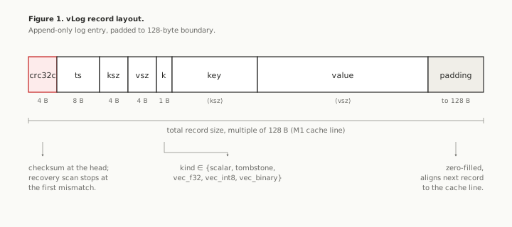
The record format is fixed. A four-byte CRC32c checksum at the head of each record permits the recovery scan to terminate at the first corruption. A timestamp, two length fields, and a kind tag follow. The payload occupies the remainder. The total record is padded to a multiple of 128 bytes, the cache line size of Apple Silicon, so that record boundaries align with the cache architecture of the target hardware.
The interesting decision was not the existence of the log but the durability barrier. A persistent write must, at some point, instruct the storage device to flush its internal buffers to non-volatile storage. On macOS the relevant primitive is F_FULLFSYNC, which is documented as guaranteeing flush to non-volatile media. The cost of F_FULLFSYNC is the round-trip latency to the SSD controller. The design documents of the project estimated this cost at approximately 20 milliseconds. The measurement returned 5 milliseconds on the target hardware, an Apple M1 with APFS over NVMe. The discrepancy is significant because the latency budget of the system is built on this number. A 5 millisecond barrier is tolerable; a 20 millisecond barrier would not have been.
A single F_FULLFSYNC per write would still produce an unacceptable throughput. The system therefore batches concurrent writes through a group commit mechanism. Multiple writes accumulate in a buffer. When the buffer reaches a configurable threshold, or a configurable time has elapsed, a single F_FULLFSYNC is issued for the entire batch. All writes in the batch receive their durability acknowledgement when the single barrier completes.
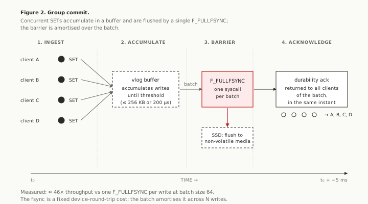
Four stages, left to right. Ingest: N concurrent SETs from independent clients enter the system. Accumulate: the requests collect in a single buffer of the vlog, bounded either by size (256 KB) or by an interval (200 µs), whichever fires first. Barrier: the buffer is flushed by exactly one F_FULLFSYNC syscall, which forces the SSD controller to commit the entire batch to non-volatile media. Acknowledge: every client of the batch receives its durability ack at the same instant, the moment the barrier returns. The fixed cost of the device round-trip is paid once, divided across N writes.
The measurement of group commit returned a throughput improvement of approximately at a batch size of 64 writes, against the same workload with one barrier per write. The number is not a surprise. The barrier is a fixed cost; amortising it over a larger batch is the standard technique. The number is recorded here because it sets the floor of the write performance of the system, and because the absence of this technique would have made the system uninteresting at any further optimisation.
Two further measurements bound the persistence layer:
- Sharding limitations: A natural extension of the single-committer architecture is to instantiate multiple committers, one per CPU core, each responsible for a partition of the key space. This was implemented. The result was unexpected. Read throughput scaled by a factor of 3.2 on four cores, which is close to the ideal speedup. Write throughput did not scale at all. A single shard committed 100K writes in 4.9 milliseconds; four shards committed 100K writes in 13.4 milliseconds. The diagnosis is that
F_FULLFSYNCis a device-global barrier. committers issuing simultaneous barriers do not parallelise; they serialise at the device. The architectural conclusion was that write scaling cannot be obtained from sharding alone; it must come from larger batches at fewer committers. The path is documented but not yet implemented as of the time of writing. - Recovery velocity: After a crash, the system must reconstruct the in-memory key index from the persisted log. The straightforward implementation is a full scan of the log at startup. On a corpus of 512 records across 16 segments, the full scan completes in 26 milliseconds. With a periodic snapshot of the index, written atomically every five minutes, the recovery scan restricts itself to the segments written since the snapshot, and completes in 1.66 milliseconds. The speedup is approximately . The snapshot mechanism was modelled on the WAL checkpoint pattern of conventional databases, adapted to the log-structured layout. The measurement was recorded as part of milestone six and remains stable.
The Cache
The persistence layer above operates with F_NOCACHE set on the file descriptors. The flag disables the operating system page cache for the log files. The choice is deliberate. The page cache of macOS is a shared resource, allocated dynamically across all processes. A process that reads its own log will, over time, occupy a portion of the page cache proportional to the size of the log. In a project whose declared concern is memory limitation, and whose target hardware is a personal laptop with a large language model resident, this is unacceptable. The page cache must remain available to the language model.
The consequence is that every read of a key incurs a disk access. A cold GET of a 4 kilobyte value takes approximately 117 microseconds on the target hardware. A warm GET, with the page cache active, would take approximately 1.4 microseconds, a difference of two orders of magnitude. The system therefore requires an explicit in-process cache, sized to a budget that the operator controls and that does not interact with the operating system page cache.
The cache implements the S3-FIFO eviction policy described by Yang and colleagues [2]. The policy is selected because it offers a hit rate comparable to LRU at lower implementation complexity and without the per-access bookkeeping cost of LFU. The cache is byte-budgeted rather than entry-budgeted. An entry-budgeted cache, in the presence of variable-sized values, can occupy a memory footprint that varies by orders of magnitude depending on the workload. A byte-budgeted cache evicts before exceeding the budget. The implementation is approximately 100 lines and uses no background eviction thread. The eviction is strict and synchronous; an insert that would exceed the budget evicts first.
The cache budget defaults to 32 megabytes per shard. The number is small by deliberate choice. The cache is supplementary; the system is designed to be correct without it, and to be performant with it within the available budget. The hit latency of the cache, measured at 5.85 nanoseconds, is below the dispatch cost of an interaction with the cache, which means the cache is not on the critical path of a cold workload and contributes only on access patterns with locality.
The Vector Tier Under Flat Scan
The system supports vector search in addition to the keyed retrieval of arbitrary payloads. The simplest configuration of vector search is a flat scan. A flat scan computes the distance from a query vector to every vector in the corpus, sorts the results, and returns the top-. The complexity is linear in the corpus size. The structure is documented in any reference on nearest neighbour search [3].
A flat scan in single precision is not viable beyond a few hundred thousand vectors at typical embedding dimensions, because the per-distance computation dominates and the linear factor becomes intolerable. The standard response is quantisation: replace the high-precision vectors with a compressed representation, compute distances on the compressed form, and re-rank the top candidates against the original precision. The system implements three quantisation tiers: single-precision float, retained as the ground truth for re-rank; 8-bit integer, with a per-axis scale calibrated from an early sample of the corpus; and 1 bit per coordinate, computed as the sign of the centred value, used as a coarse proxy.
The distance kernels are implemented in NEON intrinsics on Apple Silicon, with a scalar fallback for portability. The cosine kernel in single precision was the first to be optimised. A naive implementation issues a single fused multiply-add per loop iteration, which creates a dependency chain that the processor cannot pipeline. The optimisation maintains four independent accumulators and reduces them at the end of the loop. The measurement returned a kernel time of 126 nanoseconds for a 1536-dimensional vector, against 442 nanoseconds for the single-accumulator version. The improvement is approximately and derives entirely from instruction-level parallelism, not from any change to the operation count.
The Hamming kernel for binary distances is similarly optimised, using vpadalq_u8 for widening accumulation, and reaches a throughput of 45 gibibytes per second on a sustained flat scan of one million 192-byte codes. The target of the project plan was 20 gigabytes per second. The achieved number exceeds it by approximately a factor of two. The flat scan over a binary tier of 200 thousand vectors completes in approximately 1 millisecond.
One unexpected finding emerged in this phase: the 8-bit integer dot product, hand-rolled in NEON, was slower than the scalar fallback. The cause is the absence of the NEON vdotq_s32 intrinsic from the Rust standard library at the time of testing. The compiler auto-vectorises the scalar version more effectively than the hand-rolled version can compensate for, because the hand-rolled version cannot use the dedicated instruction. The dispatch logic therefore routes the 8-bit dot product to the scalar implementation on Apple Silicon, which is the wrong instruction for the hardware but the right instruction for the available toolchain. The structural workaround is the subject of an open contribution to the Rust ecosystem, documented in the previous post in this series.
The recall of the int8 tier against the float ground truth is empirically 1.0 on a thousand-vector corpus at dimension 128, with re-rank at the top- stage. The compression is a factor of four against single precision; the loss of accuracy is below the measurement noise. The binary tier loses more, but recovers the exact nearest neighbour at top-1 through re-rank, which is the property the system requires.
The structural ceiling of flat scan is approximately one million vectors at the latencies the system targets. Beyond that scale, the linear cost of the scan exceeds the budget. A graph index is required.
The Vamana Graph
The graph index is constructed by the Vamana algorithm, introduced by Subramanya and colleagues [4] under the name DiskANN. The construction proceeds in two passes. Each pass examines every node, computes its distances against a candidate set, and selects a bounded number of neighbours by an algorithm called RobustPrune. The first pass operates at , which produces a graph optimised for recall on the immediate neighbourhood. The second pass operates at , which extends the graph with long-range edges that accelerate the traversal across the embedding space. The combination yields a graph in which the greedy walk from any starting node terminates within a small number of steps at a neighbourhood close to the query.
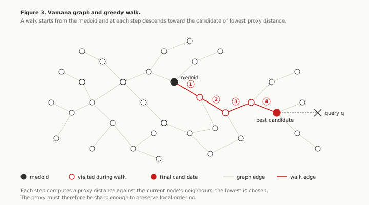
The serving operation is a greedy beam search. The walk begins at a fixed entry point, the medoid of the corpus. At each step, the walk evaluates the proxy distance from the query to each of the neighbours of the current node, selects the one with the smallest proxy distance, and advances. The walk terminates when no neighbour improves the distance, or when a configurable bound on the number of expansions is reached.
The walk does not return the final answer. It returns a candidate set. The proxy distance used during the traversal is computed on a quantised representation of the vectors, held in memory for speed. The quantisation is lossy by construction. A candidate set produced from a lossy proxy contains, in general, the true neighbours of the query but in an ordering perturbed by the quantisation error. The exact ordering, and therefore the correct top-, requires a second stage.
The second stage is a re-rank against the original full-precision vectors. The full-precision vectors are not held in memory; they are stored on disk in a separate file, arranged by node identifier. The retrieval system reads only the small number of vectors corresponding to the candidate set, computes the exact cosine distance in float against the query, sorts the resulting distances, and returns the top-. The number of disk reads is bounded by the candidate set size, typically one hundred at the default configuration. The cost is dominated by sequential disk bandwidth and is amortised over the search operation as a whole.
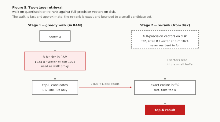
The two-stage architecture is the property that permits the memory budget to be expressed entirely in terms of the quantised tier. The full-precision vectors are sized at 4 kilobytes per vector at dimension 1024, or 4 gigabytes at one million vectors. If they were resident in memory, no quantisation would matter; the float representation would dominate. Their residence on disk is what makes the 8-bit tier the relevant quantity for the resident-set calculation. The re-rank pays its cost in disk reads, which are bounded; the walk pays its cost in proxy distance computations, which are not bounded but which operate on the smaller representation. The decomposition is the standard pattern of the DiskANN paper and is faithfully implemented here.
The recall at against brute-force ground truth, measured on SIFT-1M, is at least 0.95 with a beam of size 100. The measurement is consistent with the published results of the Vamana paper, which is the property the construction was selected for.
The graph index introduces a memory requirement that the flat scan did not have. The graph itself, stored as a fixed-degree adjacency list, occupies approximately 260 bytes per node at the default degree of 64. For one million nodes, the graph alone is 260 megabytes. The proxy tier, used to direct the greedy walk, is also resident in memory, because the cost of a disk access per step would exceed the latency budget of a query by two orders of magnitude. The 8-bit tier at dimension 1024 occupies 1024 bytes per vector, or 1 gigabyte at one million vectors. Adding the cache, the process overhead, and the index metadata, the total resident set approaches 1.3 gigabytes.
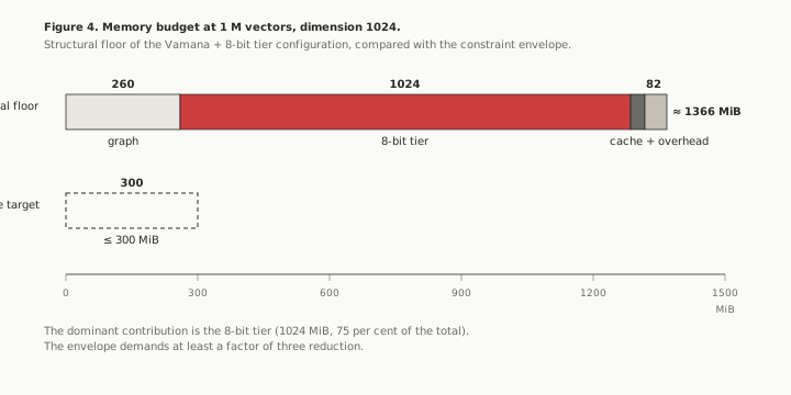
This number is the point at which the work of the previous post in this series began. The constraint envelope established in the first post permits a resident set in the low hundreds of megabytes. The substrate, by the end of milestone seven, produces a resident set approximately five times larger. The factor is the gap that the gates were intended to close.
The State at the Threshold
The system at this point was a functioning database. The persistence layer was correct under crash and recovered from snapshots in milliseconds. The cache absorbed the locality of realistic workloads without exceeding its budget. The flat scan operated at a throughput within an order of magnitude of the silicon ceiling on the kernels for which it was built. The Vamana graph delivered the recall and latency that the dominant techniques in the literature claim. None of these components is original work. Each is documented in the literature, with the citations recorded below, and each was implemented as a faithful execution of the prior art under the operational constraints of the project.
The work that began at this threshold was different. The dominant techniques produced a resident set of approximately 1.3 gigabytes per million vectors. The constraint envelope demanded approximately 300 megabytes. The reduction was the subject of the eleven hypotheses recorded across this post series. Five are documented in the previous post. Seven are documented in the next. One survived.
The substrate, as described above, did not change as the hypotheses unfolded. The persistence layer, the cache, the flat scan, the graph construction, all remained as the gates were tested. Each falsified hypothesis was a proposed amendment to the substrate. Each amendment was removed when it failed. The substrate is therefore the part of the system whose decisions were taken without the formal apparatus of pre-registered gates, on the basis of well-established prior art and routine measurement. The gates began at the point where the prior art ran out.
References
[1] Lu, Lanyue; Pillai, Thanumalayan Sankaranarayana; Arpaci-Dusseau, Andrea C.; Arpaci-Dusseau, Remzi H. “WiscKey: Separating Keys from Values in SSD-Conscious Storage.” Proceedings of the 14th USENIX Conference on File and Storage Technologies (FAST ‘16), 2016.
[2] Yang, Juncheng; Zhang, Yazhuo; Qiu, Ziyue; Yue, Yao; Rashmi, K. V. “FIFO Queues are All You Need for Cache Eviction.” Proceedings of the 29th Symposium on Operating Systems Principles (SOSP ‘23), 2023.
[3] Wang, Mengzhao; Xu, Xiaoliang; Yue, Qiang; Wang, Yuxiang. “A Comprehensive Survey and Experimental Comparison of Graph-Based Approximate Nearest Neighbor Search.” Proceedings of the VLDB Endowment, vol. 14, no. 11, 2021.
[4] Subramanya, Suhas Jayaram; Devvrit; Kadekodi, Rohan; Krishaswamy, Ravishankar; Simhadri, Harsha Vardhan. “DiskANN: Fast Accurate Billion-point Nearest Neighbor Search on a Single Node.” Advances in Neural Information Processing Systems 32, NeurIPS 2019.